Step 5: Predict with a pretrained model

In this step, you learn how to predict new examples using a pretrained model. A saved model can be used in multiple places, such as to continue training, to fine tune the model, and for prediction.

Prerequisites

Before you begin the procedures here, run .. _crash_course_train: to train the network and save its parameters to file. You use this file to run the following steps.

from mxnet import np, npx, gluon, image
from mxnet.gluon import nn
from IPython import display
import matplotlib.pyplot as plt
npx.set_np()

To start, copy a simple model’s definition by using the following code.

net = nn.Sequential()
net.add(nn.Conv2D(channels=6, kernel_size=5, activation='relu'),
        nn.MaxPool2D(pool_size=2, strides=2),
        nn.Conv2D(channels=16, kernel_size=3, activation='relu'),
        nn.MaxPool2D(pool_size=2, strides=2),
        nn.Dense(120, activation="relu"),
        nn.Dense(84, activation="relu"),
        nn.Dense(10))

In the previous step, you saved all parameters to a file. Now load it back.

net.load_parameters('net.params')

Predict

Remember the data transformation you did for the training step? The following code provides the same transformation for predicting.

transformer = gluon.data.vision.transforms.Compose([
    gluon.data.vision.transforms.ToTensor(),
    gluon.data.vision.transforms.Normalize(0.13, 0.31)])

Use the following code to predict the first six images in the validation dataset and store the predictions into preds.

mnist_valid = gluon.data.vision.datasets.FashionMNIST(train=False)
X, y = mnist_valid[:10]
preds = []
for x in X:
    x = np.expand_dims(transformer(x), axis=0)
    pred = net(x).argmax(axis=1)
    preds.append(int(pred))

Finally, use the following code to visualize the images and compare the prediction with the ground truth.

_, figs = plt.subplots(1, 10, figsize=(15, 15))
text_labels = ['t-shirt', 'trouser', 'pullover', 'dress', 'coat',
               'sandal', 'shirt', 'sneaker', 'bag', 'ankle boot']
display.set_matplotlib_formats('svg')
for f, x, yi, pyi in zip(figs, X, y, preds):
    f.imshow(x.reshape((28,28)).asnumpy())
    ax = f.axes
    ax.set_title(text_labels[int(yi)]+'\n'+text_labels[pyi])
    ax.title.set_fontsize(14)
    ax.get_xaxis().set_visible(False)
    ax.get_yaxis().set_visible(False)
plt.show()

Predict with models from Gluon model zoo

The LeNet, trained on FashionMNIST, is a good example to start with. However, it’s too simple to predict real-life pictures. In order to save the time and effort of training a large-scale model from scratch, the Gluon model zoo provides multiple pre-trained models. For example, with the following code example, you can download a pre-trained ResNet-50 V2 model that was trained on the ImageNet dataset.

net = gluon.model_zoo.vision.resnet50_v2(pretrained=True)

You’ll also need to download the text labels for each class, as in the following example.

url = 'http://data.mxnet.io/models/imagenet/synset.txt'
fname = gluon.utils.download(url)
with open(fname, 'r') as f:
    text_labels = [' '.join(l.split()[1:]) for l in f]

Downloading synset.txt from http://data.mxnet.io/models/imagenet/synset.txt...

The following example shows how to select a dog image from Wikipedia as a test, download and read it.

url = 'https://upload.wikimedia.org/wikipedia/commons/thumb/b/b5/\
Golden_Retriever_medium-to-light-coat.jpg/\
365px-Golden_Retriever_medium-to-light-coat.jpg'
fname = gluon.utils.download(url)
x = image.imread(fname)  # TODO, use npx.image instead

Downloading 365px-Golden_Retriever_medium-to-light-coat.jpg from https://upload.wikimedia.org/wikipedia/commons/thumb/b/b5/Golden_Retriever_medium-to-light-coat.jpg/365px-Golden_Retriever_medium-to-light-coat.jpg...

Following the conventional way of preprocessing ImageNet data, do the following:

1. Resize the short edge into 256 pixes.
2. Perform a center crop to obtain a 224-by-224 image.

x = image.resize_short(x, 256)
x, _ = image.center_crop(x, (224,224))
plt.imshow(x.asnumpy())
plt.show()

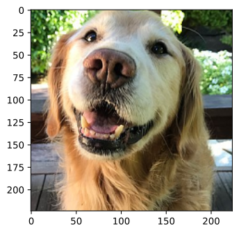
Now you can see it is a golden retriever. You can also infer it from the image URL.

The next data transformation is similar to FashionMNIST. Here, you subtract the RGB means and divide by the corresponding variances to normalize each color channel.

def transform(data):
    data = np.expand_dims(np.transpose(data, (2,0,1)), axis=0)
    rgb_mean = np.array([0.485, 0.456, 0.406]).reshape((1,3,1,1))
    rgb_std = np.array([0.229, 0.224, 0.225]).reshape((1,3,1,1))
    return (data.astype('float32') / 255 - rgb_mean) / rgb_std

Now you can recognize the object in the image. Perform an additional softmax on the output to obtain probability scores. Print the top-5 recognized objects.

prob = npx.softmax(net(transform(x)))
idx = npx.topk(prob, k=5)[0]
for i in idx:
    print('With prob = %.5f, it contains %s' % (
        prob[0, int(i)], text_labels[int(i)]))

With prob = 0.98323, it contains golden retriever
With prob = 0.00729, it contains English setter
With prob = 0.00297, it contains Irish setter, red setter
With prob = 0.00224, it contains cocker spaniel, English cocker spaniel, cocker
With prob = 0.00147, it contains Labrador retriever

As can be seen, the model is fairly confident that the image contains a golden retriever.

Next Steps

You might find that both training and prediction are a little bit slow. If you have a GPU available, learn how to accomplish your tasks faster in Step 6: Use GPUs to increase efficiency.